Improving Count Query Performance with Statistical Approximations

A recurring use-case I’ve come across is supporting queries that offer paginated selections of records, where users can supply filters and navigate to different pages (e.g., a query that would show the first hundred transactions in the past year at a particular restaurant, then the next hundred). Supporting these queries can prove challenging and books such as High Performance MySQL and MongoDB The Definitive Guide offer a number of performance optimization techniques. However, different tactics (e.g., limiting the count, caching the count, computing a different count) are only appropriate in some cases, and I’ve had to work with cases where users need to supply arbitrary filters and these tactics didn’t address all the needs of our users (in particular understanding the scale and size of the data).

The challenge is that if the DBMS has \(m\) records in general and \(n\) records that match a filter, then determining the count of records can be \(O(\operatorname{lg}(m)+n)\). This is because while it can find matching records in \(O(\operatorname{lg}(m))\) time¹, to determine the count involves actually scanning the index or table which is \(O(n)\). When there are lots of matching data this can be prohibitively expensive. What follows is a description of a way to get a pretty good approximation in \(O(\operatorname{lg}(m))\).

I should say that before you apply this you should look at your query plans, and depending on the DBMS you are using this might not be necessary. At least with versions of Mongo in use at time of writing this is useful, however to be honest I’m not sure why the Query Planner doesn’t make better use of indexes to do this effectively². I did find this whole idea and exploration neat in and of itself and thought I would share.

I will also say that before you read this, it has been 13 years since my last statistics class so some of the notation might be incorrect.

Intuition

Imagine you are in line to enter a building, and you can’t see how many people are in the line, but you know the line is sorted in alphabetical order. If you go say to the 20th person in line and ask their name, it seems intuitive that if that person’s name is James Flinders, there are probably fewer people in line than if the 20th person’s name is Bob Smith. If we wanted to actually compute an estimate we might say that since J is the 10th of 26 letters of the alphabet, and since James was 20th in line that there are maybe \(\frac{26}{10} \times 20=52\). In the line with Bob we might say that B is the 2nd letter and so estimate the size \(\frac{26}{2} \times 20=260\). Of course there are a few problems with this, the first is that names aren’t uniformly distributed, the second being that just dividing the size that way is entirely unmotivated.

Database indexes backed by B-Trees and other structures are often very performant in retrieving the first n records that match some properly, in sorted order. The fact that these queries can be performant even when full COUNT queries (which might need to scan every matching row) might not be can be used to our advantage to gain an estimate of the full size without having to actually retrieve all the data.

Leveraging UUIDs³

Many systems, including the system that I currently develop use a UUID to identify records (e.g., f81d4fae-7dec-11d0-a765-00a0c91e6bf6). If you use UUIDv4⁴ you can treat the bits⁵ as being entirely random (uniformly).

We can use this random value to obtain a value analogous to our name above:

import "strconv"

func SampleFromUUIDStr(uuid string) float64 {
    // first 12 hex chars = 48 bits
    v, _ := strconv.ParseUint(uuid[:12], 16, 48)
    return float64(v) / float64(0xFFFFFFFFFFFF)
}

The above code takes the first 12 characters of a UUID, and effectively generates a uniformly distributed random number between 0 and 1, we denote this distribution as \(U(0,1)\).

Obtaining an Approximation

/* Obtain the 128th record. */
SELECT `film_id` 
FROM `movies` 
WHERE film_location = 'Vancouver'
ORDER BY `film_id`
LIMIT 1
OFFSET 127

The above query will be performant provided you have a compound index over film_location,film_id ⁶. It will essentially give you the 128th UUID in sorted order that matches the condition of the query.

To obtain an estimate \(\hat{n}\) for the number of records \(n\) you simply compute the value \(x\) above, and plug in $k$ where k is the index you sampled (in this case \(k=128\)), into the formula:

\[\hat{n} = \frac{k}{x}-1\]

So for example here are some UUIDs, the resulting \(x\), and the estimated total number of records, if that UUID was the 128th record:

UUID	\(x\)	Estimated number of records (k=128) \(\hat{n}=\frac{128}{x}-1\)
00068db8-bac7-439b-8cec-705a4b4644ad	0.0001	1,279,999
0010624d-d2f1-4094-a988-48411db887e5	0.00025	511,999
003126e9-78d4-400b-be14-9811b7ac5b02	0.00075	170,665
00418937-4bc6-4c84-86da-488a2e5eb1ca	0.001	127,999
00da6e75-ff60-4403-b299-00ffea5d6074	0.003333	38,402
01b4dceb-fec1-4fc3-87a8-b5832bf53d5a	0.006666	19,200
028f5c28-f5c2-44ad-b657-75a85d430461	0.01	12,799
19999999-9999-48ab-bb28-86ff4ce38de2	0.1	1,279
33333333-3333-481d-a11f-8a40f217a488	0.2	639
4ccccccc-cccc-4e44-9ad2-a64a49d86ca0	0.3	425
66666666-6666-48b0-92ee-7db1c62eb752	0.4	319
7fffffff-ffff-4a7d-8da5-d1019591e180	0.5	255
99999999-9999-48a3-afa6-6a933a454988	0.6	212
b3333333-3332-47b5-9082-2b056bb907ba	0.7	181
cccccccc-cccc-4c80-9409-ffbc6ce14884	0.8	159
e6666666-6665-485a-98ce-d548b051a72a	0.9	141

There are a few practical considerations, what if you don’t get any results, or x=0 or x=1. In practice, we compute exact counts up to some value, say 500, and only if the value is greater than that, compute an approximation, as for the edge cases, they are very unlikely (1 in 282 trillion), and if you are worried about them, you can just nudge the value for x slightly (or use the first 16 characters which for technical reasons should never result in 0 or 1). The performance of the above query is \(O(k)\), but for our purposes k is a constant, so \(O(1)\).

Statistical Background

So where did this come from and how good is this estimate? Well it comes from Order Statistics. The k-th order statistic is the k-th smallest value over a set of samples. So for example, if we sample a random variable \(X\) 4 times and get the values 6, 9, 3, 7, then we would get four values \(X_n\) and when sorted the order statistics \(X_{(n)}\), as shown:

\(n\)	\(X_n\)	\(X_{(n)}\)
1	6	3
2	9	6
3	3	7
4	7	9

Each \(X_n\) has the same distribution of \(X\), but the distribution of \(X_{(n)}\) varies with \(n\)⁷.

If you have a set of random variables \(U_1, U_2, ...\) that are distributed \(U(0,1)\), then the order statistic \(U_{(1)}\) is the lowest of those values, and \(U_{(k)}\) is the kth lowest value in the set. According to Wikipedia, the distribution of \(U_{(k)} = \operatorname{Beta}(k ,n+1-k)\), where Beta is the Beta Distribution. The Beta distribution, denoted \(\operatorname{Beta}(\alpha,\beta)\) has parameters \(\alpha, \beta\) and a mean \(\mu=\frac{\alpha}{\alpha+\beta}\).

Substituting in our parameters, gives us:

\[\mu = \frac{k}{k+n+1-k} = \frac{k}{n+1}\]

We can use our sample \(x\) as an estimate for the mean \(\hat{\mu}\), to estimate \(n\) with some rewriting ⁸:

\[\hat{n} = \frac{k}{\hat{\mu}}-1\]

How Good of an Estimate is it

I wanted to understand how good of an estimate the formula was empirically⁹ and how that impacts the choice of k¹⁰. I ran some Monte Carlo simulations, for differing sizes of \(n \in [10000, 81920000], k \in [1,16384]\), generating a value from \(U(0,1)\) \(n\) times, sorting and then sampling the kth value, for each pair (n,k) 20,000 samples were obtained.

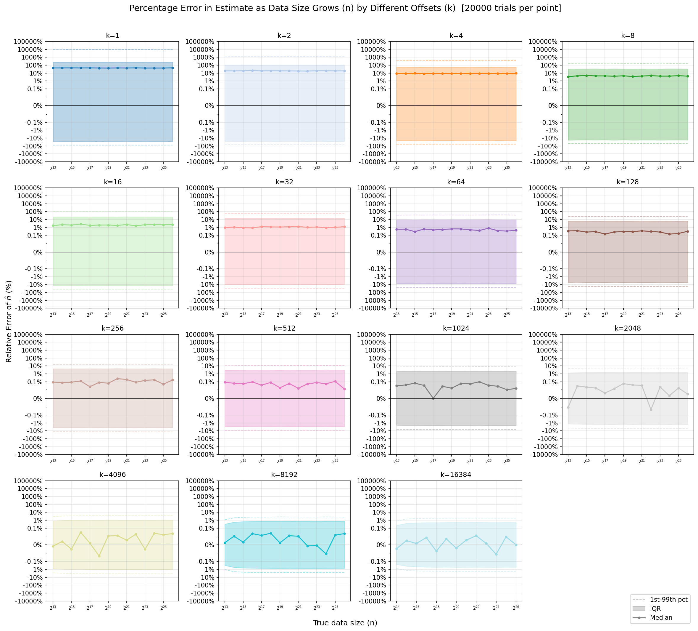
Shown above is for different k values what the relative error \(\frac{\hat{n}-n}{n}\) is as the number of samples (in our case matching records) increases. It shows the median, the interquartile range (50% of the time the sample falls in this value), and the two outer dashed lines represent where the value fell 98% of the time.

Some important conclusions:

1. The accuracy of the estimate is largely independent of the number of matches.
2. Using a value of around \(k=64\) gives you something that 98% of the time will be +/- 50% of the true value.
3. Using a value of around \(k=16384\) gives you something that 98% of the time will be +/- 2% of true value.
4. Very small values of \(k\) are terrible estimates.

Looking at the graphs, you might wonder why the median error is seemingly above zero, and notice that the range of the data tends to be an overestimate of the data (i.e., it’s not symmetric about 0%). I believe this is the result of the fact that mean and median of the beta distribution are not the same, and that the distribution is not symmetric, and is not something to be concerned about.

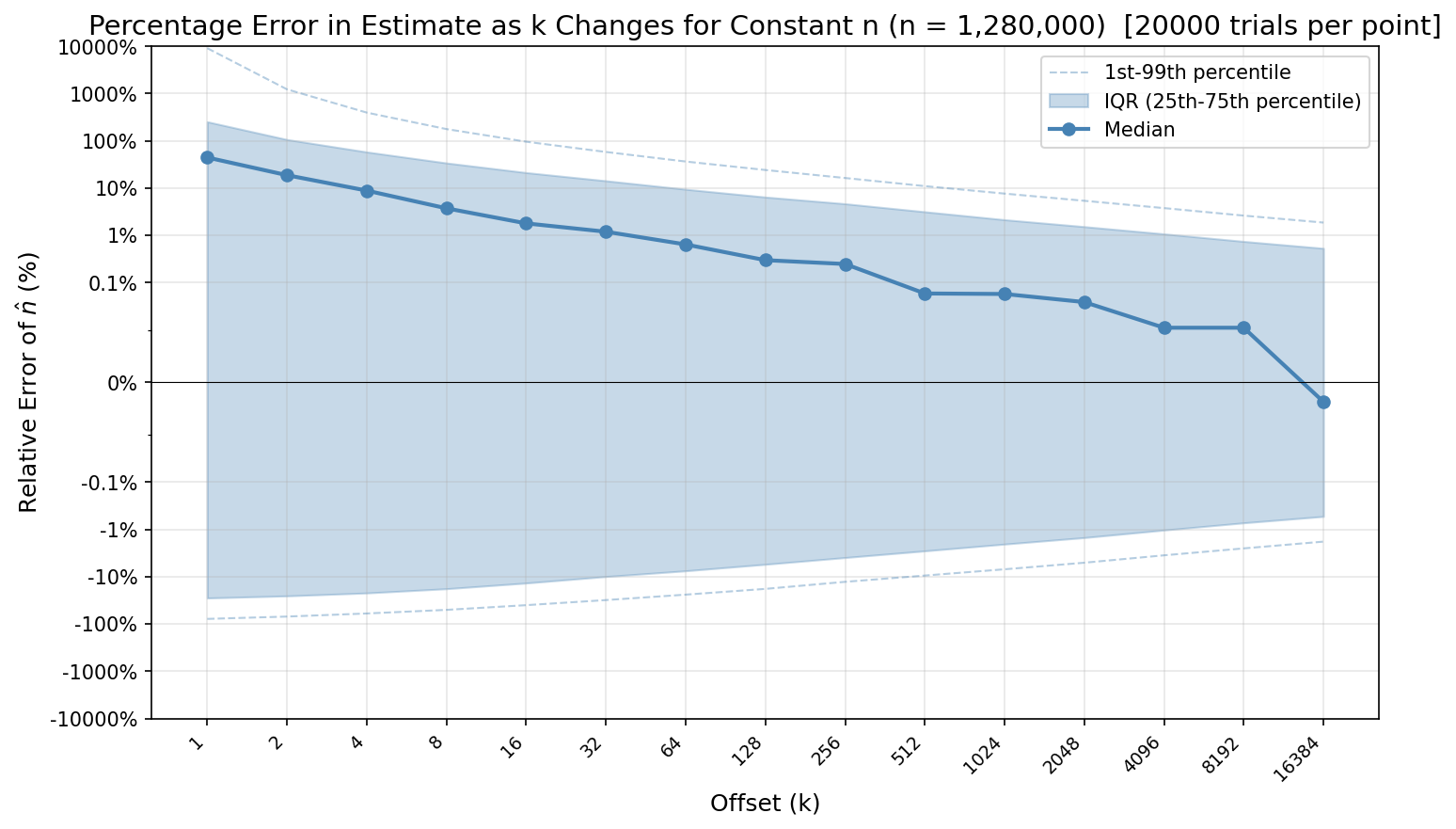
Below shows a particular size of matches, and shows how the error decreases as you change your offset.

Interested readers can also see absolute (instead of relative) plots here and here, as well the data generation and visualization code.

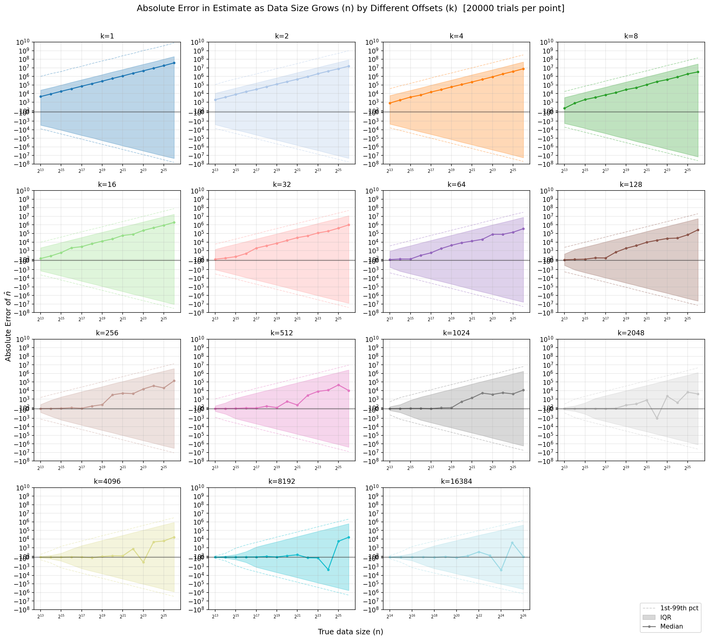
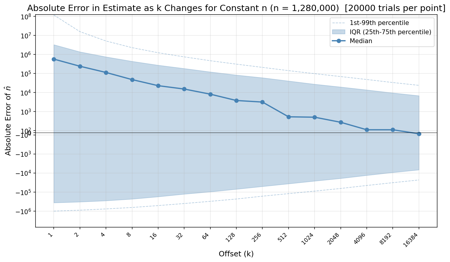
Possible Future Improvements

Typically, with LIMIT and OFFSET queries the database needs to do all the work to retrieve LIMIT + OFFSET rows and then throws away the OFFSET results. In this case, it seems like we might be able to get a better estimate by not just pulling in the kth value, but using all the values. My initial experiments with this didn’t work however, and it might be because the samples are not independent (in other words you can’t assume that both \(U_{(k)}\) and \(U_{(k+1)}\), have Beta distributions, because \(U_{(k+1)}\) becomes conditional on the value of \(U_{(k)}\)¹¹.

While I have no doubt it’s possible to improve things for this problem, if more accurate estimates are needed, we would just spend 10 seconds to increase the value of k and probably not dig out the statistics textbooks.

Summary

So in summary if your DBMS is slow to compute COUNT queries with filters then to provide a performant estimate:

1. Define a compound index over the filter conditions and a uniformly distributed random value (such as a UUID, or just a float).
   • Note: An auto incrementing id, many other versions of UUID (such as v1) or others derived from Mongo’s default _id will not work.
2. Pick some k maybe around 128 (depending on how good of an estimate you need), and grab the kth record from the DB ordered by the random value (e.g., the UUID), converting that value to a random number \(x\) between 0,1.
3. The estimated count is then \(\frac{k}{x}-1\).

1. Assuming the right indexes exist. ↩

2. In particular, if you are searching for records with say \(x=4\), why the query seems to find the first x=4, and then iterate over all rows with that property. It seems like it could also find the first \(x > 4\), and then simply count how many records are between by examining the B-Tree. ↩

3. If your system doesn’t use UUIDs you could still use the ideas here, by simply storing a random float on each record to achieve the same end. Admittedly, it’s a lot less elegant. ↩

4. At a glance v5 and v3 would probably also work, v7 may also have some random bits that could be used. ↩

5. Not all bits in a UUIDv4 are guaranteed to be random, in UUIDv4 only 122 bits are random. For the most part, I will just ignore the details. ↩

6. You should consult your DBMS documentation for the specifics, but assuming your index is backed by an B-Tree this should be pretty quick to execute. ↩

7. There is an interesting 3 blue one brown video that talks about the distribution of the second order statistic of two variables here: A bizarre probability fact. ↩

8. Whether this is a good estimator for n, is maybe beyond my depth. ChatGPT suggests this estimator is consistent with the MLE estimate in this case, but I didn’t verify this. ↩

9. It’s likely possible to derive expressions for the variance of \(\hat{u}\), but it’s more algebra than I wanted to present (or do :)). ChatGPT suggests the variance is defined for k > 2, and decreases at a rate of \(\frac{n}{\sqrt{k}}\), but I didn’t check this. It further suggested that the relative error for n much larger than k tends to wash out and so becomes independent of n. ↩

10. In systems I’ve worked with choices of k even at 10,000 are fine, the problems came when we had matches that were in the 100,000, or million range. ↩

11. I highly suspect that this and related problems are well studied in statistics. ↩